
So you’ve spent weeks building a dataset and coding up a neural network. You’ve trained the model, and are getting less-than-stellar results. What do you do next?
Deep learning is often seen as a black box, and I’m not going to argue with this view — what sense can you make of tens of thousands of learned parameters?
But the black-box view poses an obvious problem for machine learning practitioners: How do you debug a model?
In this post, I’ll walk through some techniques we’ve used at Cardiogram to debug DeepHeart, a deep neural network to predict diseases using data from the Apple Watch, Garmin, and WearOS devices.
At Cardiogram, we believe that constructing DNN architectures isn’t alchemy, it’s engineering.
#1: Predicting Synthetic Outputs
Test the abilities of your model by predicting a synthetic output task built from your input data.
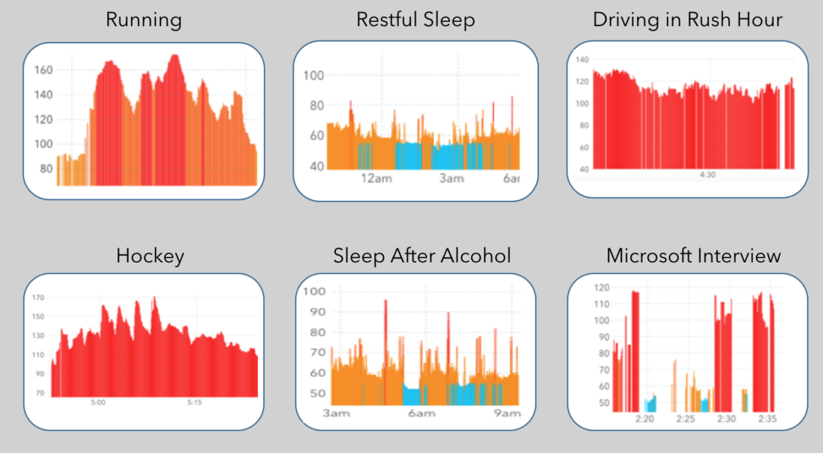
We applied this technique when constructing a model to detect sleep apnea. Existing literature on sleep apnea screening used the difference in standard deviation of heart rate between daytime and nighttime as a screening mechanism. Thus we created a synthetic output task for each week of input data:
std(daytime HRs) — std(nighttime HRs)
In order to learn this function, a model needs to be able to:
- Distinguish day from night
- Remember data from several days in the past
Both of these are pre-requisites to predicting sleep apnea, so one of our first steps in experimenting with a new architecture is to check if it is able to learn this synthetic task.
You can also use synthetic tasks like this in a form of semi-supervised training by pre-training the network on the synthetic task. This is useful when labeled data is scarce, but you have a lot of unlabeled data.
#2: Visualizing Activations
It is difficult to understand the internals of a trained model. How do you make sense of thousands of matrix multiplications?
In this excellent Distill paper, the authors analyzed a handwriting model by graphing cell activations in a heatmap. We found this to be an excellent way to “pop open the hood” of your DNN.
We examined the activations of several layers of our network, hoping to find some semantic properties, for example cells that activate when the user is sleeping, working out, or anxious.
The code to extract activations from a model is simple in Keras. The below code snippet creates a Keras function last_output_fn that obtains a layer’s output (it’s activations), given some input data.
from keras import backend as K

def extract_layer_output(model, layer_name, input_data):
  layer_output_fn = K.function([model.layers[0].input],
                               [model.get_layer(layer_name).output])

  layer_output = layer_output_fn([input_data])

  # layer_output.shape is (num_units, num_timesteps)
  return layer_output[0]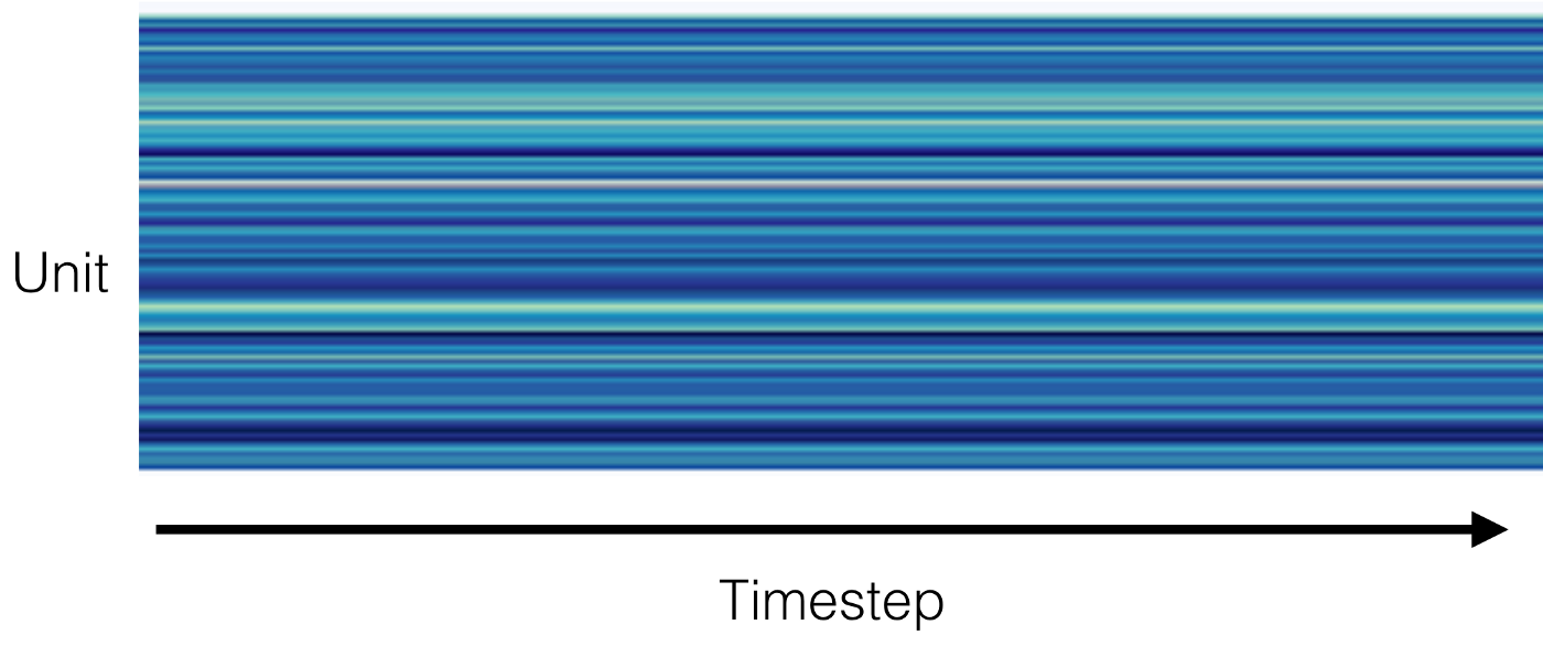
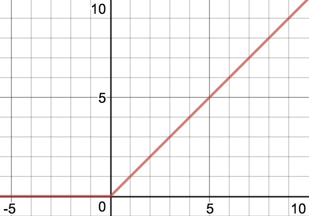
This architecture uses ReLU activation function, which outputs zero when the input is negative. This is indeed what is happening, though at an earlier layer in the network.
At some point in training, large gradients caused all bias terms of a layer to become very negative, making the input to the ReLU function very negative. Thus this layer emitted all zeros, and because the gradient of the ReLU is zero for inputs less than zero, the problem could not be fixed through gradient descent.
When one convolutional layer emits all zeros, cells in the subsequent layer output the values of their bias terms. This is why each unit of this layer outputs a different value — their bias terms differ.
We fixed this problem by replacing the ReLU with a Leaky ReLU, which allows gradients to propagate even when the input is negative.
We didn’t expect to find dead neurons in this analysis, but of course the hardest bugs to find are the ones you’re not looking for.
#3: Gradient Analysis
Gradients are useful for more than optimizing your loss function. In gradient descent, we compute Δloss with respect to Δparameter. In general though, gradients compute the effect of changing one variable on any other. And because gradient computation is necessary for gradient descent, frameworks like TensorFlow include functions to compute gradients.
We used gradient analysis to determine whether our DNN could capture long term dependencies in the data. The inputs to our DNN are very long: 4096 timesteps of heart rate or step count data. It’s very important that our architecture be able to capture long term dependencies in this data. For example, heart rate recovery time is predictive of diabetes. This is the amount of time it takes to get back to your resting heart rate after working out. To compute this, a DNN must be able to compute your resting heart rate, and to remember the time when you ended your workout.
A simple measure of whether a model can track long term dependencies is to check the impact of each timestep of input data on the output prediction. If the later timesteps have dramatically larger impact, the model is likely not effectively using earlier data.
The gradient we’d like to compute is Δoutput with respect to Δinput_t, for all timesteps t. Here is example code to compute this using Keras and TensorFlow:
def gradient_output_wrt_input(model, data):
  # [:, 2048, 0] means all users in batch, midpoint timestep, 0th task (diabetes)
  output_tensor = model.model.get_layer('raw_output').output[:, 2048, 0]
  # output_tensor.shape == (num_users)

  # Average output over all users. Result is a scalar.
  output_tensor_sum = tf.reduce_mean(output_tensor)

  inputs = model.model.inputs # (num_users x num_timesteps x num_input_channels)
  gradient_tensors = tf.gradients(output_tensor_sum, inputs)
  # gradient_tensors.shape == (num_users x num_timesteps x num_input_channels)

  # Average over users
  gradient_tensors = tf.reduce_mean(gradient_tensors, axis=0)
  # gradient_tensors.shape == (num_timesteps x num_input_channels)
  # eg gradient_tensor[10, 0] is deriv of last output wrt 10th input heart rate

  # Convert to Keras function
  k_gradients = K.function(inputs=inputs, outputs=gradient_tensors)

  # Apply function to dataset
  return k_gradients([data.X])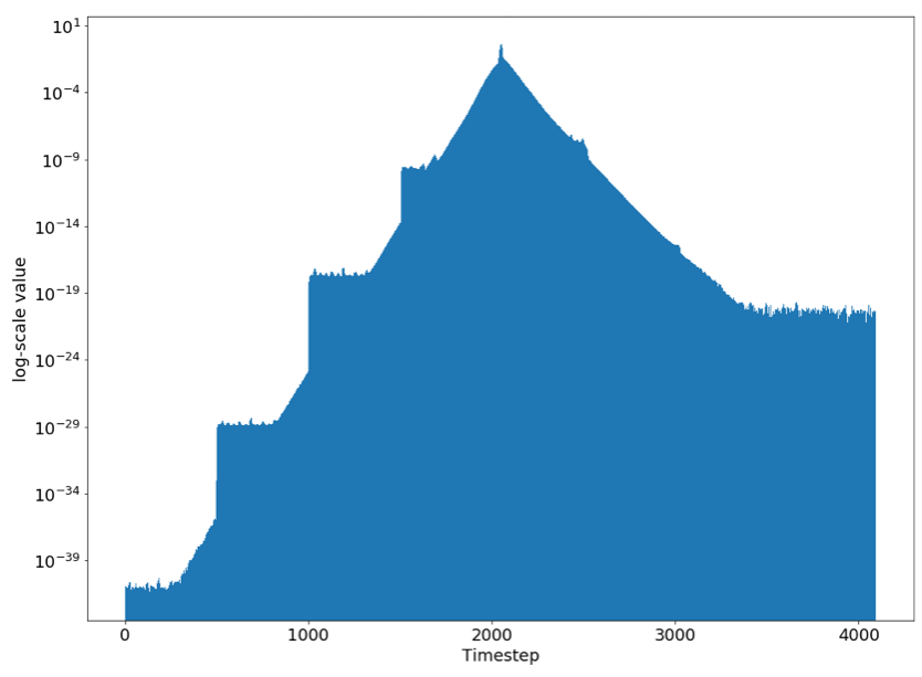
Notice that the y axis is log-scale. The gradient of the output with respect to the input at timestep 2048 is 0.001. But the gradient with respect to the input timestep 2500 is one million times smaller! Through gradient analysis, we discovered that this architecture cannot capture long term dependencies.
#4: Analyze Model Predictions
You’re probably already analyzing model predictions, at the very least by looking at metrics like AUROC and Mean Absolute Error. There’s a lot more analysis you can run to understand you model’s behavior.
For example, we were curious whether our DNN was actually using the heart rate input to generate predictions, or whether it was leaning heavily on provided metadata — we initialize the LSTM state with user metadata like age and sex. To understand this, we compared the model outputs to a logistic regression model trained on the metadata.
The DNN takes in one week of user data, so in the below scatter plot, each dot is a user week.
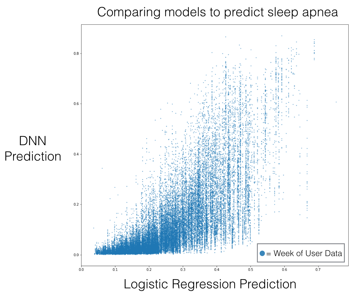
This plot invalidated our hypothesis, as the predictions aren’t highly correlated.
In addition to aggregate analysis, it can be instructive to look at examples of your top wins and losses. For a binary classification task, you’ll want to look at the most egregious false positive and false negative (ie cases where the prediction is farthest from the label). Try to identify loss patterns, then filter out those patterns patterns that also occur in your true positives and true negatives. e
Once you have a hypothesis on a loss pattern, test it through stratified analysis. For example, if the top losses were all from the 1st generation Apple Watch, we could calculate accuracy metrics on the set of users in our tuning set with 1st generation Apple Watches and compare these with metrics computed on the rest of the tuning set.
I hope these tips will help you in debugging your model! If you have any more tips, leave a comment — we’d love to learn from you.
Want to help us? Cardiogram is hiring! If you’ve got design chops, front end engineering skills, or research experience in machine learning, let’s talk.
—
This post is adapted from a talk we gave at O’Reilly AI in September of this year.